VSR: Virtual studio 3-D reconstruction and relighting with real image-based relighting

Showcase Paper Info Datasets Appendix Code
^Contents

1. More on Related Works


~Missing Image~

1. More on Inverse Rendering

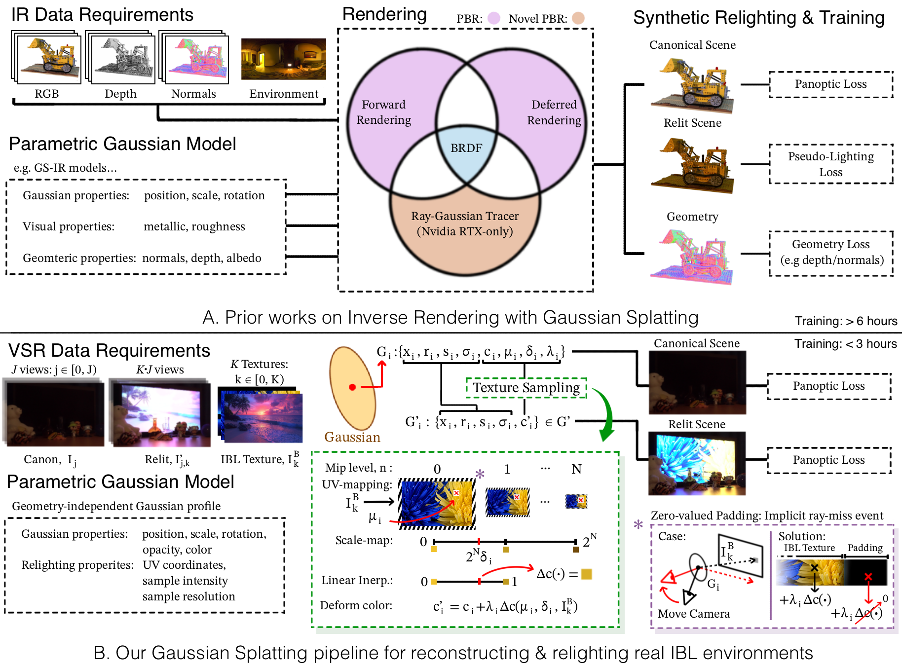
In the figure above we compare the IR and VSR data requirements, generic Gaussian primitives, rendering pipeline and training scheme. There are clear differences regarding representation, data needs and loss functions. Notably, our method acts independent of Gaussian geometry, does not rely on priors and can be trained using the simple panpotic loss function. Futhermore, our method does not require custom CUDA/RTX code and uses the well documented gsplat rasterizer.


2. Unconstrained Illumination in Photo Collections (UIPC)

UIPC research focuses on 3D scene relighting for unconstrained photo collections. This mainly involves reconstructing landmarks from data that is scraped from social media websites, so contains seasonal appearance captured over different periods of the day and year. Here, 3D relighting pipelines are expected to interpolate between the variable lighting as well as deal with various geometric capture conditions. UIPC shares similarity with our VSR paradigm, as VSR also ingests a dataset with variable light conditions. The difference lies with the research objective, as UIPC pipelines mainly focus on dealing with explicit geometric uncertainties related to the unconstrained photo collections. For example, the XX landmark dataset is composed of images scraped from social media so the data contains distractors, like transient humans or vehicles or animals. Instead, our method aims to capture implicit geometric phenomena to support unseen lighting conditions, i.e. when a new background texture is introduces. As a result, UIPC research is mainly focused on dealing with temporal distractors that arise from, As the main paradigm of VSR regards the approach to IBL texture sampling, there is not much inspiration that can gained from comparing VSR to UIPC.


3. Gaussian Splatting Texture Enhancement (GTE)

GTE research mainly focuses on anti-aliasing problems for generic scene reconstruction, not relighting. GTE focuses on novel ray-Gaussian intersection schemes that allow for Gaussian sub-sampling - enhancing the expressivity of the scene. Thus, GTE research remains unrelated to the VSR texture sampling. However, TexGS proposes a Gaussian sub-sampling method that samples a ground truth RGBA texture per-Gaussian. TexGS adopts a color deformation scheme akin to dynamic GS reconstruction, replacing the temporal color residual with a view-dependent color residual. Inspired by this work, we extend the deformation model by introducing an intensity parameter that modifies the magnitude of the deformation, independent of IBL texture. This essentially models a static exposure setting, which future work could explore for scene editing applications.

2. More on Designing Proxy Baslines


The figure below visualizes the rendering process of the proxy baselines (2A-2D) presented in the main paper.

~Missing Image~

A. Bilinear Sampling Smoothness

Basline A represents the vanilla approach to texture sampling that is used in practice. The code below demonstrates how this sampling method is applied.


def sample_tex(I, uv, s, num_levels=3):
    uv = 2.*uv -1. # Normalize sample coordinates [-1, 1]
    uv = uv.unsqueeze(0).unsqueeze(0) # Reshape
    return F.grid_sample(I.unsqueeze(0), uv, mode='bilinear', align_corners=False, padding_mode='border').squeeze(2).squeeze(0).permute(1,0)


B. Local Smoothness via TriPlanes

This method is inspired by IR works that used neural fields for modelling various lighting/surface parameters. We also chose to use this as it related to various potential options for extending our VSR approach for dynamic scenes. 2B uses the same texture sampling scheme as 2A with the following approach for learning the additional lighting parameters.


self.sample_decoder = nn.Sequential(nn.ReLU(),nn.Linear(net_size, net_size),nn.ReLU(),nn.Linear(net_size, 16*2))
self.invariance_decoder = nn.Sequential(nn.ReLU(),nn.Linear(net_size, net_size),nn.ReLU(),nn.Linear(net_size, 16*1))    
...
features = self.grid(rays_pts_emb[:,:3])

uv = torch.sigmoid(self.sample_decoder(features)).view(-1, 2, 16)
invariance = torch.sigmoid(self.invariance_decoder(features)).view(-1, 1, 16)


C. Mahalanobis Screen-space Smoothness

This method is inspired by deferred rending techniques that process lighting in image space. The code below shows how this is done and uses the same texture sampling function as in A (adapted for handling I_uv as uv coordinate inputs).


I_lamba = gsplat.render(..., color=invariance)
I_mu = gsplat.render(..., color=mu)
I_base = gsplat.render(..., color=colo)
render = I_base + I_invariance*sample_tex(uv=I_mu, ...)


D. MipMaps for Multi-scale Textures

This method is an multi-scale extension of 2A inspired by classical graphics approaches to sampling textures using mipmaps. The code below shows how sample_tex() is evolved for our mipmap approach.


def generate_mipmaps(I, num_levels=3):
  maps = [I]    
  for _ in range(1, num_levels):
      maps.append(F.interpolate(I, scale_factor=0.5, mode='bilinear', align_corners=False, recompute_scale_factor=True))
  return maps
def sample_mipmap(I, uv, s, num_levels=3):
    maps = generate_mipmaps(I, num_levels=num_levels) # Generate downsampled images
    uv = (2.*uv -1.).unsqueeze(0).unsqueeze(0) # Normalize and reshape
    
    # Determine the lower and upper bounds of the scaling parameter
    L = s*(num_levels-1.)
    lower = torch.floor(L).long().clamp(max=num_levels-1)
    upper = torch.clamp(lower + 1, max=num_levels-1)
    s_interp = (L - lower.float())

    # Sample mipmaps
    mip_samples = torch.empty((N, num_levels, 3), device=s.device)    
    for idx, map in enumerate(maps):
        mip_samples[:, idx] = F.grid_sample(map, uv, mode='bilinear', align_corners=False, padding_mode='border').squeeze(2).squeeze(0).permute(1,0)

    # For each gaussian linearly interpollate based on s_interp and upper and lower.
    gather_idx_low  = lower.view(N, 1, 1).expand(-1, 1, 3)
    gather_idx_high = upper.view(N, 1, 1).expand(-1, 1, 3)
    colors_low  = torch.gather(mip_samples, 1, gather_idx_low).squeeze(1)   # [N,3]
    colors_high = torch.gather(mip_samples, 1, gather_idx_high).squeeze(1) 

    return (1. - s_interp) * colors_low + s_interp * colors_high
        

3. Per-Dataset and Per-Scene Results for Baseline Experiments

1. Full Novel View and Lighting Synthesis (NVLS), Novel View Synthesis (NVS) and Novel Lighting Synthesis (NLS) Results

The test data can be split into three categories:
(1) Novel view and light synthesis (NVLS) where novel views and novel light conditions are tested
(2) Novel view synthesis (NVS) where novel views and trained light conditions are tested
(3) Novel light synthesis (NLS) where trained views and novel light conditions are tested
Switch between "NVLS", "NVS" and "NLS" tabs in the sheet below to view the per-dataset and per-scene results for each baseline.

2. Side-By-Side Test Videos for the Baseline Experiments

Below we provide videos for a handful of the NVLS, NVS and NLS video results. Note that we compile the videos per-datset. Each tile is essentially it's own 1080p video, so youtube will compress this even with 4k settings. You can click here for the original image-based side-by-side results. More videos are avalibale on the main page.

C. Extended Analysis of Full Baseline Results

The test data can be split into three categories:

4. Ablation Experiments

1. Full per-scene metric results for the ablations on Dataset 3

The NVLS results for each ablation experiment is provided in the google sheet below. The video results and extended descriptions/analysis of each ablation experiment is provided in each section below. The first presents analysis on experiments (i-ii). The second presents the statistical approach and statistical outcomes of experiment (iii), where we evaluate the effect of selecting K=1 IBL scenes based on texture statistics. The third presents the additional ablation results, evaluating the impact of reformulating the training of the canonical scene based on different practical scenarios.

2. Side-By-Side Test Videos and Extended Analysis for Experiments (i-ii)

Each tile is essentially it's own 1080p video, so youtube will compress this even with 4k settings. You can click here for the original image-based side-by-side results.

Here is lies...


3. Ablating the Canonical Scene

In the carousel below, we present two important ablations concerning the canonical scene
(a) The case when no "unlit" references are avaliable so one of the lit scenes acts as the canonical scene
(b) The case when the canonical scene is left un-constrained by removing the canonical loss from training
As done previously, we test this on Dataset 3 and show the video results below.

...

5. Extending VSR Capabilities


1. Statistical Approach and Results for (iii): Optimizing performance via statistically-drive texture selection

In the carousel below, we present the outcomes and insights of experiment (iii). This concerns the capture scenrio where only 1x IBL scene/background is captured, as was done in experiment (ii.a). However, we question whether a texture could be selected to optimize for VSR quality. To accomplish this we evaluate two important traits associated with spatially-varying RIC-IBL textures:
(1) The frequency density of the image, i.e. how varied is the frequency distribution of the texture?
(2) The texture regularity/uniformity, i.e. how unique are local image patches?
For (1) we use the energy function for the Garbor-Wavelet coefficients to indicate the variance and magnitude of texture-frequencies, in a single metric. The Garbor-Wavelet is typically used for natural images, over e.g. Fourier or other Wavelet schemes.
For (2) we use the homoeneity heuristic from the Grey-Level Co-occurent Matric (GLCM). This is another common scheme for assessing the regularity/uniformity of a texture. A set of heuristics are avaliable under the GLCM algorith, though we find the results are relatively similar, so we select the homogeneity metric for this paper. The GLCM algorithm is reliant on computing metrics based on filter direction and scale. This is essentially the direction along the image should we move to compare the current pixel-patch to the next, and how far we should move. In this paper we evaluate four directions, 0deg, 45deg, 90deg, 135deg, and four distances 1 pixel, 2 pixels and 4 pixels. The GLCM Scikit-learn package handles this all for us.

The results show that selecting the right texture can have an large impact on both reconstruction and lighting quality. This experiment effectively shows that textures can be statistically selected to boost VSR performance. Carrying this into the VS use-case, this insinuates that backgrounds can be designed for VSR prupose. In layman terms, directors would no longer need to make decisions about VFX and scene lighting before or during filming. If they capture scenes for VSR rather than for the final pixel, important creative decisions could be made later in the process with much more flexibility and fine-grained control. Especially considering that VSR inherits the editability and AOVs associated with Gaussian Splatting tools and research.


6. More on Subjective Study

7. More on Limitations and Future work


1. Static VSR Problems

Not all filmmaking is dynamic. In VS production, the range applications exceeds human-centric capture. Hence, there is value is developing robust static VSR pipelines.

A good use case for this is car advertisement, where cars are placed within a VS volume to simulate driving in various foreign locations. Through VS production, numerous costs linked to trasnportation, insurance and hiring car-specific camera hardware can be avoided. Pre-production planning is also simplified as directors no longer need to consider location-specific challenges. Still, VS sets are expensive to hire, various shot types are still challenging to achieve, and baked lighting for highly reflective and transparent surfaces (i.e. cars) are non-trivial to edit in post. Hence, VSR provides a clear solution to reducing VS productions costs by only having to capture the scene once and also support downstream video/shot editing. However, we chose this case because it also highlights flaws in our current VSR approach that need to be developed in future work. The results from our model show that one of the largest challenge with VSR is rendering high-resolution reflections in regions where Gaussian distribution is sparse. This mostly concerns the relighting of highly reflective transparent surfaces, so would present major problems when filming cars for advertisement using a VS stage.

We believe this issue mainly lies with our choice of adaptive Gaussian densification scheme. We use the vanilla approach that instances points based on the gradient changes propagrated from the reconstruction loss. Hence, image-regions with greater reconstruction errors garner greater attention. However, this method of instancing new Gaussians relies on spliting and cloning pre-existing Gaussians. This presents problems in regions with sparse Gaussians, such as those relating to transparent object. Hence, during training our VSR pipeline is unlikely to populate these spatial regions. This highlights the need for content-aware densifications schemes.

Past this we believe that the initialization of per-Gaussian texture sample coordinates could be improved. When viewing the novel view synthesis results with a moving camera we notice view-dependent flickering artifacts. This occurs when the view-dependent change in texture sample coordinates is sensitive and the IBL sample scale is low, i.e. when the Gaussian samples a high-resolution mipmap. For IBL textures high local frequency patterns, this can be detrimental to viewing smoothness. In part this is a dataset limitation - as we only use 18 cameras for training, sparse-view reconstruction problems arise leading to view-dependent overfitting. Thus, future work may want to explore methods of smoothing view-dependent features to suppress flickering artifacts.


2. Dynamic VSR Problems

Developing a dynamic VSR pipeline reguires first understanding the four types of illumination events. First, illumination can change due to changes in RIC-IBL texture. Second, illumination can change depending on the viewing angle. Third, illumination can change depending on the global position of the object within the scene. Fourth, illumination can change depending the objects local orientation. In the paper, we deal with disentangling the first two types of lighting event. The third and fourth events arise when dealing with dynamic or editable static scenes.

Dynamic VSR pipelines that deal with all four events could concievable take a number of approaches:
(1) Modelling 3D neural exposure and texture sampling fields with occlusion awarness
(2) Implicitly modelling per-Gaussian temporal lighting and shadow features

Regarding option (1), future work could rely signed distance fields (SDF) typically found in neural surface reconstruction research. The challenge here would be to adapt the per-Gaussian texture sampling and exposure parameters (proposed in the paper) as a 3D neural field, such that as an object moves within the 3D field the lighting reponse changes. This problem can be simplified by assuming that the VS LED wall is static, hence the 3D lighting field can be modelled as time-independent. For example, using a neural radiance field (ie.e. a coordinate MLP) would only require inputting the current position to return the gamma and mu lighting parameters prodposed in the paper. To deal with local temporal events (i.e. the fourth type of illumination event), a dynamic signed distance field could then be employed to handle lighting-based occlusions. This would ideally modify the lighting reponse from the 3D light fields to account for dynamic shadows and highlights. For filmmaking, we believe this options is the strongest option as, ideally, this solution models 3D lighting field independent of the scene composition. Hence, the step towards instancing new objects, removing objects, or moving objects is trivialized as the 3D light field and occlusion model should be capable of handling these types of event.

On the other hand, option (2) may provide a stronger approach to fitting a dynamic scene for cases where geometry editing is not desired/necessary. The challenge here would be to discover per-Gaussian representation that inherits the prior accomplishments of dynamic GS while also handling with local lighting changes. A naive solution to this may involve the hexplane representation which could be used to approximate residual changes in gamma and mu w.r.t time, such that c' = c + gamma(t)*delta_c(mu(t), I_k^B). We could then implicitly deal with occlusions by introducing an additional temporal indensity parameter that models c'' = psi(t) * c'. Still, work would need to be done towards designing a training strategy that is capable of disentangling/constraining gamma(t) and psi(t). Otherwise this naive solution would be prone to overfitting the psi(t) parameter as it undergoes a larger degre of gradients flow in comparison to gamma(t), during backpropagation.


References


[]